MasteringElectronicsDesign.com:Build an Op Amp SPICE Model from Its Datasheet – Part 1 and Part 2 show you how to build an Op Amp SPICE model based on the manufacturer’s datasheet. We talked about modeling the offset voltage, the input resistance and capacitance both common-mode and differential, the output resistance and the frequency domain behavior.
In Part 2, we left off at the open-loop bode plot. We saw that it resembles the datasheet. However, our op amp example, ADA4004 from Analog Devices, shows an extra pole after 1 MHz. Indeed, the phase starts dropping after 1 MHz and becomes 45 degrees at 17 MHz. Therefore, we need another pole in our model at 17 MHz.
Introducing the Second Pole
The pole can be introduced using the same technique we used in Part 2. We will use an RC Norton source. Since the DC open-loop gain is already set by the first pole, we only need to make sure that the choice of current and resistor does not affect the DC gain. This second pole influence has to be only at high frequencies. At low frequencies its gain should be 1, so that the overall open-loop gain remains 500000.
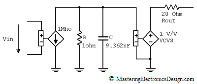
Figure 1 shows the Norton source with a pole at 17 MHz.
Figure 1
The components are calculated as follows. The resistor is calculated first, so that the DC gain is 1. The Voltage-Controlled-Current-Source (VCCS) gain is chosen to be 1 Mho. This is a trans-conductance amplifier, so the units are in Mho (inverse of Ohm). Therefore, for a gain of one, the resistor has to be 1ohm.
Then the capacitor is calculated based on the pole we need at 17 MHz. The RC expression is:
With R2 = 1 Ohm, the capacitor is C2 = 9.362 nF. (The beauty of these models is that we do not need to be concerned with choosing standard values for capacitors and resistors. )
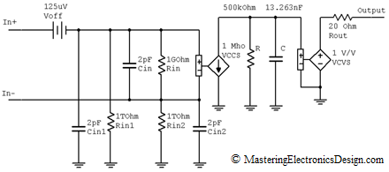
Now, let’s insert this pole in our model. As we built this model, we arrived at the version shown in Part 2, Figure 4, and it is shown again here, in Figure 2 for convenience.
Figure 2
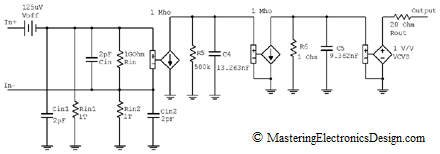
We will insert the second pole circuitry between the capacitor C and the Voltage-Controlled-Voltage-Source (VCVS) at the model output. We can do this, because the two poles are isolated between them. Why? The VCCSs have high input/output impedance, so each pole impedance at any frequency cannot influence the behavior of the other pole. In doing so, we take full advantage of the ideal components we use in this model. They are not real components, but they model a mathematical behavior of the real circuit, and this is what we want to accomplish.
The new circuit is shown in Figure 3. Click the figure to expand it.
Figure 3
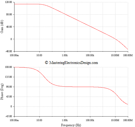
And now comes the test. If we simulate this model the open loop Bode plot resembles exactly the body plot shown in the ADA4004 datasheet, Rev. F, Figure 14. The Bode plot is shown in Figure 4.
Figure 4
As expected, the first pole is at 24 Hz, where the phase becomes 135 deg (45 deg phase shift versus the phase at low frequencies). The second pole is at 17 MHz, where the phase becomes 45 deg. With this technique one can add other poles or even zeros if necessary, to accurately simulate the circuit behavior. In Part 4 we will introduce the input bias currents and offset current.


